
Personal Comments
In this series I attempt to collect results concerning stabilities in topological data analysis. Researches in this direction has been increasing dramatically in recent years. Without doubt there will be more in the future. However, the best will not appear until one really understands all the progresses.
The first stability theorem in TDA is proved by David Cohen-Steiner, Herbert Edelsbrunner, John Harer. It asserts that the bottleneck distance between two persistence diagrams is bounded by the \(\infty\)-norm of tame functions. They soon generalized this result to \(L_p\) cases for tame Lipschitz functions (see here). This theorem is fundamental in TDA. And the idea is also direct -- counting points in persistence diagrams. We sketch the procedure in the following.
Recall that a persistence diagram is a multiset in the extended plane \(\bar{\mathbb R}=\mathbb R\cup \{\infty\}\). A tame function \(f:X\to\mathbb R\) defined on a topological space induces a finite filtration \[ \emptyset=f^{-1}((-\infty,a_0])\to\cdots\to f^{-1}((-\infty,a_i])\to\cdots\to f^{-1}((-\infty,a_n])=X. \] Each \(a_i\) is called a homological critical value. Thus, at \(a_i\) the homotopy type of the sublevel sets of \(f\) is changed. Tameness means that it changes finite types. Let \(b_i<a_i<b_{i+1}\) be interleaved sequences. The maps \(H_k(f^{-1}(-\infty,b_i])\to H_k(f^{-1}(-\infty,b_{i+1}])\) are not isomorphisms. For simplicity, let us drop the subscript \(k\), and denote the homology group by \(H(b_i)\). Let \(f_{x,y}\) denote the map \(H(x)\to H(y)\). The image of \(f_{x,y}\) is denoted by \(H(x,y)\). Set \(\beta(x,y)={\rm dim} H(x,y)\). We can define the multiplicity of a point \((a_i,a_j)\) in persistence diagram \(D(f)\) as \[ \mu(i,j)=\beta(b_{i-1},b_j)-\beta(b_i,b_j)+\beta(b_i,b_{j-1})-\beta(b_{i-1},b_{j-1}). \] Then the total multiplicity (or size) of the persistence diagram over the diagonal is \[ \#(D(f)-\Delta)=\sum_{i<j}\mu(i,j). \] Next we count multiplicities in different areas on the diagram.
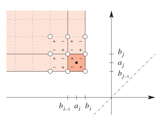
Let \(Q_x^y=[-\infty,x]\times[y,\infty]\) be the closed upper left quadrant. k-Triangle Lemma asserts that for \(x<y\) different from homological critical values, then \[ \#(D(f)\cap Q_x^y)=\beta(x,y). \] The proof is shown in the following figure. Note that the small square with plus and minus notations explains the multiplicity at a point. When summing over, plus and minus cancels.
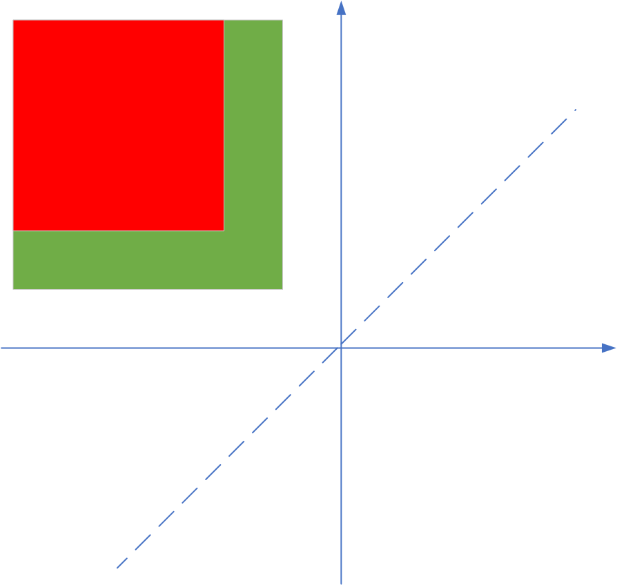
Let \(f\) and \(g\) be two tame functions on the same topological space. Let \(\epsilon=\|f-g\|_{\infty}\). We want to compare the multiplicities of quadrants for \(f\) and \(g\). In fact, the Quadrant Lemma asserts that \[ \#(D(f)\cap Q_{x-\epsilon}^{y+\epsilon})\le \#(D(g)\cap Q_x^y). \] Symmetrically, we also have \[ \#(D(g)\cap Q_{x-\epsilon}^{y+\epsilon})\le \#(D(f)\cap Q_x^y). \] Intuitively, when we shift the quadrant upper left by \(\epsilon\), the multiplicity decreases.
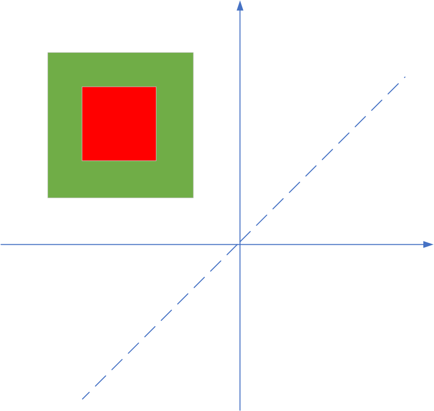
Let \(R=[a,b]\times[c,d]\) be a closed rectangle where \(a<b<c<d\). Let \(R_{\epsilon}=[a+\epsilon,c-\epsilon]\times[c+\epsilon,d-\epsilon]\) be a smaller rectangle. The Box Lemma asserts that the points in the smaller box have less multiplicities. \[ \#(D(f)\cap R_{\epsilon})\le \#(D(g)\cap R). \] Similarly, the positions of \(f\) and \(g\) can be exchanged in the inequality.
Let \(A\) and \(B\) be multisets in the extended plane. The Hausdorff distance between \(A\) and \(B\) is defined as \[ d_{\mathcal H}(A,B)=\max\{\sup_x\inf_y\|x-y\|_{\infty},\sup_y\inf_x\|y-x\|_{\infty}\}, \] where \(x\in A\) and \(y\in B\). Using box lemma, we can easily deduce that \[ d_{\mathcal H}(D(f),D(g))\le \|f-g\|_{\infty}, \] since for each point in \(D(f)\), there is at least one point in \(D(g)\).
The final step is to generalize the inequality to bottleneck distance. By definition, the bottleneck distance between \(A\) and \(B\) is \[ d_{\mathcal B}(A,B)=\inf_{\gamma}\sup_x\|x-\gamma(x)\|_{\infty}, \] where \(\gamma:A\to B\) is bijection. Note that \(D(f)\) contains the diagonal with infinite points. Therefore, the bottleneck distance is well defined. Since there are finitely many points off the diagonal in a persistence diagram, we can assume that \(f\) and \(g\) are so close that in a square of length \(\|f-g\|_{\infty}\) there is only one point in \(D(f)\). On the other hand, by box lemma we also have a point in \(D(g)\). This enables us to construct a bijection but the distance is \(\|f-g\|_{\infty}\). For general \(f\) and \(g\), we interpolate piecewise linear functions and use triangle inequality to pass the conclusion to \(\hat{f}\) and \(\hat{g}\). In a word, we obtain the main theorem
Let \(X\) be a triangulable space with continuous tame functions \(f,h:X\to \mathbb R\). Then the persistence diagrams satisfy \(d_{\mathcal B}(D(f),D(g))\le\|f-g\|_{\infty}\).
In proving the quadrant lemma and box lemma, one notice that there is an interleaving phenomenon of the level sets of \(f\) and \(g\). This interleaving is generalized to modules, which is purely algebraic. See F. Chazal etc. for references.