
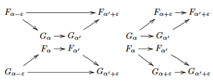
One observes that when proving the \(L^{\infty}\) stability theorem, the functions \(f\) and \(g\) provide nothing but an interleaved inclusion of level sets \(f^{-1}((-\infty,a])\subseteq g^{-1}((-\infty,a+\epsilon])\subseteq f^{-1}((-\infty.a+2\epsilon])\). This further gives the following commutative diagram.
Instead of taking functions and spaces into account, let us forget about geometry and work on algebra directly. That is, we consider two sequences of modules such that the above diagram commutes. In the terminology of F. Chazal etc., the two sequences of modules are called (weakly/strongly) \(\epsilon\)-interleaved. It would be no surprise that the distance between two persistence diagrams are bounded by \(\epsilon\). However, when working in an algebraic approach, we can drop many restrictions on spaces and functions. Furthermore, we generalize the definition of persistence diagrams hence the conclusion is also strengthened.
Let \(A\) be a subset of \(\mathbb{R}\) and \(R\) be a field. A persistence module \(\mathcal{F}_A\) is a collection of vector spaces \(\{F_{\alpha}\}_{\alpha\in A}\) together with linear maps \(\{f_{\alpha}^{\alpha'}:F_\alpha\to F_{\alpha'}\}\) such that for any \(\alpha\le \alpha'\le\alpha''\), we have \(f^{\alpha''}_\alpha=f^{\alpha''}_{\alpha'}\circ f^{\alpha'}_\alpha\) and \(f^\alpha_\alpha=id_{F_\alpha}\). A persistence module is called tame if each vector space is of finite dimension. In the following all persistence modules are assumed to be tame.
Let \(\Delta\) be the diagonal \(\{(x,x)|x\in\bar{\mathbb{R}}\}\) and \(\Delta_{+}\) be the space on and upon the diagonal \(\{(x,y)|y\ge x\}\). If \(A\) is discrete with no accumulation point, we can define the persistence diagram of \(\mathcal{F}_A\) to be a multiset \(\mathcal{DF}_A\) in \(\Delta_{+}\). The points in \(\mathcal{DF}_A\) are in the form \((\alpha,\alpha')\) where \(\alpha\le \alpha'\in A\). For each point on the diagonal \(\Delta\) the multiplicity is \(\infty\). For each point off the diagonal, the multiplicity is \[ \mu(\alpha_i,\alpha_j)=\left\{\begin{array}{l}rank(f^{\alpha_{j-1}}_{\alpha_i})-rank(f^{\alpha_j}_{\alpha_i}),\alpha_i=\inf A\\ rank(f^{\alpha_{j-1}}_{\alpha_i})-rank(f^{\alpha_j}_{\alpha_i})+rank(f^{\alpha_j}_{\alpha_{i-1}})-rank(f^{\alpha_{j-1}}_{\alpha_{i-1}}),else\end{array}\right. \] This coincides with the previous definition. To define the persistence diagram of an arbitrary index set needs some preparation.
Let \(B\subseteq A\) be a subset with no accumulation point. Let \(\Gamma_B\) be the grid \(\{(\beta_i,\beta_j)|\beta\in B\}\). To each grid \(\Gamma_B\) is associated with a B-pixelization map \(pix_B:\Delta_{+}\to \Gamma_B\cup\Delta\). If a cell does not hit the diagonal, \(pix_B\) sends each point in the cell to the upper right grid point. If a cell hits the diagonal, then each point is send to the closest point on the diagonal.
Since we can always pick out a subsequence in the persistence module, it is natural to define the persistence diagram of \(\mathcal{F}_A\) through an approximation of \(\mathcal{DF}_B\) with \(B\subseteq A\).
Let us say a persistence module \(\mathcal{F}_B\) is \(\epsilon\)-periodic is the index set \(B=\alpha_0+\epsilon \mathbb{Z}\). Then we have the following lemma
Let \(B,C\subseteq A\). The pixelization map \(pix_B\) defines a multi-bijection between \(\mathcal{DF}_{B\cup C}\) and \(\mathcal{DF}_B\). Furthermore, for any \(\epsilon\)-periodic persistence modules \(\mathcal{F}_B\) and \(\mathcal{F}_C\), we have \(d_B^{\infty}(\mathcal{DF}_B,\mathcal{DF}_A)\le \epsilon\).
Therefore, Set \(\epsilon=2^{-n}\), the persistence diagrams \(\mathcal{DF}_{B_n}\) will form a Cauchy sequence under bottleneck distance. The diagram of \(\mathcal{F}_A\) is defined to be the limit of this sequence.
As mentioned in the beginning, the interleaving between level sets of spaces become interleaving between persistence modules. Two persistence modules \(\mathcal{F}_{\mathbb{R}}\) and \(\mathcal{G}_{\mathbb{R}}\) are strongly \(\epsilon\)-interleaved if there exists two families of homomorphisms \(\{\phi_\alpha:F_\alpha\to G_{\alpha+\epsilon}\}\) and \(\{\psi_{\alpha}:G_\alpha:\to F_{\alpha+\epsilon}\}\) such that the diagram in the beginning commutes. Then we have the following theorem about stability
Let \(\mathcal{F}_{\mathbb{R}}\) and \(\mathcal{G}_{\mathbb{R}}\) be tame persistence modules. If \(\mathcal{F}_{\mathbb{R}}\) and \(\mathcal{G}_{\mathbb{R}}\) are strongly \(\epsilon\)-interleaved, then \(d_B^{\infty}(\mathcal{DF}_{\mathbb R},\mathcal{DG}_{\mathbb R})\le \epsilon\).
The proof of this theorem is lengthy. However, for persistence diagrams with finite points off the diagonal, the idea is nothing but an algebraic analogy to the geometric stability proof -- one constructs a family of persistence modules \(\mathcal{H}^s\) which interpolates between \(\mathcal{F}_{\mathbb{R}}\) and \(\mathcal{G}_{\mathbb{R}}\). Then, for close enough \(\mathcal{H}^s\) and \(\mathcal{H}^{s'}\) the distance between persistence diagrams can be bounded by the Box Lemma. The bound for \(\mathcal{DF}_{\mathbb R}\) and \(\mathcal{DG}_{\mathbb R}\) is obtained by triangle inequality.
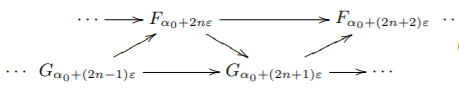
For general persistence diagram (with possibly infinite points off the diagonal), more techniques are involved. Two persistence diagrams \(\mathcal{F}_A\) and \(\mathcal{G}_B\) are weakly \(\epsilon\)-interleaved if there exists some \(\alpha_0\) such that \(\alpha_0+2\epsilon\mathbb Z\subseteq A\) and \(\alpha_0+\epsilon+2\epsilon\mathbb Z\subseteq B\) and there are homomorphisms such that the following diagram commutes
One needs to prove a weakly stability theorem to assist the strong one.
Let \(\mathcal{F}_{A}\) and \(\mathcal{G}_{B}\) be tame persistence modules. If \(\mathcal{F}_A\) and \(\mathcal{G}_B\) are weakly \(\epsilon\)-interleaved, then \(d_B^{\infty}(\mathcal{DF}_A,\mathcal{DG}_B)\le 3\epsilon\), and the bound is tight.
To obtain the \(3\epsilon\) bound we need to investigate the pixelization map carefully. But we can use the pixelization lemma to prove a loose bound easily. Let \(\mathcal{H}\) be the persistence module \[ \cdots\to G_{\alpha_0+(2n-1)\epsilon}\to F_{\alpha_0+2n\epsilon}\to G_{\alpha_0+(2n+1)\epsilon}\to\cdots \] Then \(\mathcal{F}_{\alpha_0+2\epsilon\mathbb Z}\) and \(\mathcal{G}_{\alpha_0+\epsilon+2\epsilon\mathbb Z}\) are subcollections of \(\mathcal{H}\). By the pixelization lemma, we have \(d_B^{\infty}(\mathcal{DF}_{\alpha_0+2\epsilon\mathbb Z},\mathcal{DG}_{\alpha_0+\epsilon+2\epsilon\mathbb Z})\le 2\epsilon\). Similarly, we have \(d_B^{\infty}(\mathcal{DF}_{\alpha_0+2\epsilon\mathbb Z},\mathcal{DF}_A)\le 2\epsilon\) and \(d_B^{\infty}(\mathcal{DG}_{\alpha_0+\epsilon+2\epsilon\mathbb Z},\mathcal{DG}_B)\le 2\epsilon\). By triangle inequality, we have the bound \(6\epsilon\).