
Let \(\mathbb X\) be a triangulable, compact metric space, \(f,g:\mathbb X\to\mathbb R\) be tame functions (that is, \(f\) and \(g\) have finitely many homological critical values.) The sublevel sets of \(f\) (resp. \(g\)) form a filtration of spaces. Using fields as coefficient groups, It gives a finite sequence of homology groups (vector spaces) in each dimension. A homology class is born if it is not an image from preceding homology groups, and is said to be died if it merges with other classes when entering succeeding homology groups. With the notion of birth and death, in each dimension one can associate \(f\) (resp. \(g\)) a multiset in the two-plane called the persistence diagram, denoted by \(D_k(f)\) (resp. \(D_k(g)\)) for \(k=0,1,\cdots\). The bottleneck distance of \(D_k(f)\) and \(D_k(g)\) is defined as \[ d_B(D_k(f),D_k(g)):=\inf_{\gamma \text{ bijection}}\sup_{x\in D_k(f)}||x-\gamma(x)||_{\infty} \] It was proved that persistence diagrams are robust to small perturbations of functions. More specifically, David Cohen-Steiner, Herbert Edelsbrunner, John Harer ('2007') proved that, for each \(k\) one has \[ d_B(D_k(f),D_k(g))\le||f-g||_\infty \] In analogy to Wasserstein distance, they note that bottleneck distance is a special case of a more general form. Let \(D(f)\) be the union of all \(D_k(f)\). Define the degree-\(p\) Wasserstein distance between \(D(f)\) and \(D(g)\) by \[ W_p(D(f),D(g))=\left[\inf_{\gamma \text{ bijections}}\sum_{x\in D(f)}||x-\gamma(x)||_\infty^p\right]^{\frac{1}{p}} \] To prove a stability result for Wasserstein distance, additional conditions are required for the space \(\mathbb X\) and functions \(f\) and \(g\). We shall explain the details about the work of David Cohen-Steiner, Herbert Edelsbrunner, John Harer, Yuriy Mileyko ('2010').
Size of triangulation.
A crucial step in proving the main theorem is to bound the number of points in the diagram whose persistence exceeds some threshold. In fact, they observed that this quantity can be controlled by the size of triangulation. That is why we need to assume the space \(\mathbb X\) is triangulable. Precisely, a triangulation of \(\mathbb X\) is a finite simplicial complexes \(K\) together with a homeomorphism \(\nu:|K|\to \mathbb X\). For a simplex $$ in \(K\) we can define its diameter \(\text{diam}(\sigma)=\max_{x,y\in\sigma}d(\nu(x),\nu(y))\). The mesh of \(K\) is defined as \(\text{mesh}(K)=\max_{\sigma\in K}\text{diam}(\sigma)\). The size of \(K\) is the number of simplices in \(K\), denoted by \(\text{card}(K)\). We are interested in the following size function \[ N(r)=\min_{\text{mesh}(K)\le r}\text{card}(K) \] A rough observation is that, \(N(r)\) is a non-increasing function, and when \(r\) tends to 0, \(N(r)\) will tend to infinity. For 'good' spaces we can estimate that the order of divergence. For example, if \(\mathbb X\) is an \(n\)-dimensional ball (or cube), then the cardinality of simplices is proportional to \(\text{vol}(\mathbb X)/r^n\). For compact Riemannian manifold of dimension \(n\) the order also holds true. This inspires to propose the 'polynomial growth' assumption: there are constants \(C_0\), \(R_0\) and \(M\) such that for \(r<R_{0}\), \(N(r)\le \frac{C_0}{r^M}\).
One clearly sees that the inequality cannot hold for all \(r>0\) since it leads to nonsense \(N(r)\to 0\) as \(r\to \infty\). In fact, the value of \(N(r)\) for large \(r\) is the minimal triangulation of the space \(\mathbb X\). Even for the simplest case, say, an \(n\)-dimensional cube, the exact value of the minimal triangulation is not completely known. (See this post) .
Lipschitz Functions
Recall that \(f:\mathbb X\to \mathbb R\) is a Lipschitz function if there is a constant \(c\) such that \(d(f(x),f(y))\le cd(x,y)\) for all \(x,y\in \mathbb X\). The infimum over all such \(c\) is called the Lipschitz norm of \(f\), denoted by \(\text{Lip}(f)\).
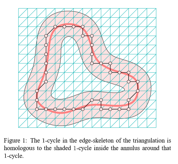
The reason to consider Lipschitz functions is that the sublevel sets of Lipschitz functions are well separated. For simplicity assume \(f\) is non-expanding, i.e. \(\text{Lip}(f)=1\). Then for \(x\in f^{-1}(a)\) and \(y\in f^{-1}(b)\) with \(a<b\) we have \(d(x,y)\ge b-a\). Furthermore, denote \(\mathbb X_a=f^{-1}((-\infty,a])\) and \(\mathbb X_b=f^{-1}((-\infty,b])\). Let \(\mathbb X_a^r=\{z\in\mathbb X|d(z,\mathbb X_a)\le r\}\) be the set of points within distance \(r\) to \(\mathbb X_a\). Then \(\mathbb X_a^{b-a}\subseteq \mathbb X_b\). This allows us to thicken the sublevel sets without breaking the order of inclusion.
Thickening a subset is helpful for us to find simplicial cycles in \(K\) that approximate singular cycles in \(\mathbb X\). This is best illustrated in the figure (copied from paper '2010')
Bounding Persistent Cycles
Fix a tame non-expanding function \(f\) on the triangulable, compact metric space \(\mathbb X\). Let \(P(f,\epsilon)\) be the number of points in the diagrams of \(f\) whose persistence exceeds \(\epsilon\). Then the Persistent Cycle Lemma claims that \(P(f,\epsilon)\le N(\epsilon)\) for any \(\epsilon\).
Proof. Let \(K\) be a triangulation such that \(\text{mesh}(K)\le \epsilon\). Let \(\alpha\) be a homological class in any dimension whose persistence exceeds \(\epsilon\). i.e. \(\text{per}(\alpha)=\text{d}(\alpha)-\text{b}(\alpha)\ge\epsilon\). Let \(z(\alpha)\) be a closed cycle in \(\mathbb X_{\text{b}(\alpha)}\). By separation of Lipschitz function, \(\mathbb X_{\text{b}(\alpha)}^{\text{b}(\alpha)+\epsilon}\subset\mathbb X_{\text{b}(\alpha)+\epsilon}\). Thus, there is a closed cycle \(\bar{z}(\alpha)\) in \(K\) which is homologous to \(z(\alpha)\) in \(\mathbb X_{\text{b}(\alpha)+\epsilon}\).
Suppose there are \(m\) points in the diagram of dimension \(l\) whose persistence exceeds \(\epsilon\). By construction, we can find \(l\) dimensional cycles \(\bar{z}_1,\bar{z}_2,\cdots,\bar{z}_m\). Assume the birth time are ordered \(\text{b}_1\le\text{b}_2\le\cdots\le \text{b}_m\). We claim that these cycles are independent. Suppose \(\bar{z}_i\) is not independent of its predecessors. i.e. \(\bar{z}_i\sim\sum_{j=1}^{i-1}\lambda_j\bar{z}_j\). In \(\mathbb X_{\text{b}_i+\epsilon}\) we have \(z_i\sim\sum_{j=1}^{i-1}\lambda_jz_j\). Without loss of generality we assume \(\text{b}_i>\text{b}_j\) for \(i>j\) (or we can put the same \(\text{b}_i\) together). By definition, this means that \(z_i\) is dead before \(\text{b}_i+\epsilon\), contradiction. By induction, these cycles are independent. Note that the number of independent cycles is bounded by the number of \(l\) dimensional simplices. Summing over we see that \(P(\epsilon,f)\) is bounded by \(N(\epsilon)\).
Estimating Persistence Moments
View a persistence diagram as a sum of Dirac measures. We want to estimate the moments \[ \text{Per}_k(f)=\sum_{x\in D(f)}\text{per}(x)^k \] Call it degree-k total persistence of \(f\). More generally, we consider the following function \[ \text{Per}_k(f,t)=\sum_{\text{per}(x)>t}\text{per}(x)^k \] From this point of view, \(P(t,f)\) is the measure of \(\{x|\text{per}(x)>t\}\). For simplicity, Let us project the diagram to the \(t\)-axis so that all functions are treated as functions on \(\mathbb R\). Then \(P(t,f)\) is a decreasing stair function. The derivative of \(P(t,f)\) with respect to \(t\) is the negative of Dirac function. Hence \[ \text{Per}_k(f,t)=\int_{\epsilon>t}-P(\epsilon,f)'\epsilon^kd\epsilon \] Integrating by parts we obtain \[ \text{Per}_k(f,t)=t^kP(t,f)+k\int_t^{\text{Amp}(f)}P(\epsilon,f)\epsilon^{k-1}d\epsilon \] where \(\text{Amp}(f)=\max f-\min f\le \text{diam}(\mathbb X)\).
But \(P(t,f)\) is bounded by \(N(t)\) and \(N(t)\) is assume to has a polynomial growth when \(t\) is small. Suppose there are constants \(C_{\mathbb X}\) and \(M\) such that when \(t\le \text{Amp}(f)\), \(N(t)\le C_{\mathbb X}/t^M\). We see that \[ \text{Per}_k(f,t)\le t^kC_{\mathbb X}/t^M+k\int_t^{\text{Amp}(f)}C_{\mathbb X}\epsilon^{k-1-M}d\epsilon \] when \(k=M+\delta\) with \(\delta>0\), \[ \text{Per}_k(f,t)\le C_{\mathbb X}\text{diam}(\mathbb X)^\delta+\frac{M+\delta}{\delta}C_{\mathbb X}\text{diam}(\mathbb X)^\delta=\frac{M+2\delta}{\delta}C_{\mathbb X}\text{diam}(\mathbb X)^\delta \] Thus we see that there is a uniform bound on \(\text{Per}_k(f,t)\) which only depends on the space \(\mathbb X\). Therefore, we abstract the following definition
Definition. A metric space \(\mathbb X\) implies bounded degree-k total persistence if \(\text{Per}_k(f)\) is uniformly bounded for all non-expanding functions.
From the discussion above, a triangulable, compact metric space with polynomial growth size of order \(M\) implies bounded degree-\((M+\delta)\) total persistence.
Wasserstein Stability
Let \(\mathbb X\) be a triangulable, compact metric space which implies bounded degree-k total persistence. \(f\) and \(g\) are two tame non-expanding functions on \(\mathbb X\). Then \[ W_p(D(f),D(g))\le C_{\mathbb X}||f-g||_\infty^{1-k/p} \] where \(p\ge k\) and \(C_{\mathbb X}\) is a constant depending only on \(\mathbb X\).
Proof. Let \(||f-g||_\infty=\epsilon\). Let \(\gamma:D(f)\to D(g)\) be a bijection such that \(d_B(D(f),D(g))=||f-g||_\infty\). Note that \(||x-\gamma(x)||\le 1/2(\text{per}(x)+\text{per}(\gamma(x)))\). Thus, \[ W_p(D(f),D(g))^p\le \epsilon^{p-k}\sum ||x-\gamma(x)||_\infty^k\le\epsilon^{p-k}/2\sum (\text{per}(x)^k+\text{per}(\gamma(x))^k) \] by the convexity of \(x^k\). The stability inequality follows.
Wasserstein Stability for Point Clouds
Recall that for a finite metric space \(X=\{x_1,x_2,\cdots,x_n\}\) with \(n\) points. We have an isometric embedding \[ \rho:X\to\mathbb (R^n,||\cdot||_\infty) \] by \(\rho(x_i)=(d_X(x_1,x_i),\cdots,d_X(x_n,x_i))\). If \(X,Y\) are finite metric spaces with Gromov-Hausdorff distance \(\epsilon\), we can find a compact metric space \(Z\) such that \(X,Y\) isometrically embed into \(Z\) with Hausdorff distance \(\epsilon\). Then we can embed \(X\cup Y\) into \(\mathbb R^{n_X+n_Y}\). The Cech filtration of \(X\) and \(Y\) are the sublevel set filtration of \(\delta_X\) and \(\delta_Y\). Note that \(||\delta_X-\delta_Y||_\infty\le\epsilon\). However, the space \(\mathbb R^{n_X+n_Y}\) is not compact. The Wasserstein stability theorem cannot apply directly.
One way to overcome this difficulty is to restrict \(\delta_X\) and \(\delta_Y\) to a subset of the total space. It is easy to check that \(X\cup Y\) is bounded by a cube of radius \(a=\min\{\text{diam}(X),\text{diam}(Y)\}+2\epsilon\). We see that this cube satisfies the polynomial growth condition \(N(r)\le C_n\frac{a^n}{r^n}\) where \(n=n_X+n_Y\) (just divide the cube into \(a^n/r^n\) small cubes where each cube can be triangulated by \(C_n\) simplices). Hence the cube implies \(k\)-total persistence with constant \(C_n a^{k}\) where \(k>n\). At this moment we can use Wasserstein stability to obtain a bound by the Gromov-Hausdorff distance of point clouds.
However, this result is not of much importance since the stability depends on the number of point clouds. The problem is that the point clouds we are considering are too general while the Wasserstein stability for spaces are restrictive. A reasonable assumption is to consider finite samples from a \(k\)-dimensional Riemannian manifold (or Finsler manifold). But one should be careful with Nerve theorem since it will not be true for general open covers.
To start up, let us consider the simplest case where point clouds are Euclidean, i.e. finite samples from Euclidean spaces. Now the embedding is fixed and Nerve theorem is true for any convex cover. The only question is to find a suitable metric for point clouds.
Let \(X,Y\) be compact subsets of \(\mathbb R^d\) where \(d\) is fixed. Let \(\mathcal E(d)\) be the Euclidean group acting on \(\mathbb R^d\). Consider the distance given by \[ d^{\mathbb R^n}_\mathcal{EH}(X,Y)=\inf_{T\in \mathcal E(d)}d^{\mathbb R^n}_{\mathcal H}(X,T(Y)) \] This distance defines a metric on the set of isometric classes of compact subsets in \(\mathbb R^n\) (see Memoli). This distance is also commonly used in image/point cloud registration problem. It is often be approximated by Iterative Closet Poing (ICP) algorithm.
Obviously \(d_\mathcal{GH}\le d_\mathcal{EH}\) and it is often the case where the inequality is strict. However, it is proved that \(d_\mathcal{EH}\le cd_\mathcal{GH}^{1/2}\) thus two distances are equivalent. For our case \(d_\mathcal{EH}\) is more convenient. Let \(a=d_\mathcal{EH}\). For any \(\epsilon>0\) we can find an isometry \(T\in \mathcal E(d)\) such that the Hausdorff distance between \(X\) and \(T(Y)\) is less than \(a+\epsilon\). Therefore, \(X\cup T(Y)\) lies in a ball of radius \(2(\max\{\text{diam}(X),\text{diam}(Y)\}+a+\epsilon)\). This ball clearly satisfies the polynomial growth condition and the distance function \(\delta_X\) restricted on the ball has the same filtration homotopy of \(\delta_X\) on the whole space. According to the Nerve theorem, the sublevel filtration of \(\delta_X\) is the Cech filtration of point clouds. Now apply Wasserstein Stability theorem and we obtain an inequality between the Wasserstein distance of Cech persistence diagrams and Euclidean-Hausdorff distance between \(X\) and \(Y\).