Informally, the problem of graph partitioning, or graph clustering, can be stated as follows: we want to partition a graph into several parts such that there are fewer edges between groups but more edges within groups. If there is a measurement on edges, i.e. the edges are weighted, then it can also be stated that we want a partition that nodes within groups are more similar. Graph partitioning can be encountered in many areas such as statistical learning, network analysis, graph learning. Other than data science, it is also related to graph theory and computer vision. One recalls that there is a classical problem called minimum cut in graph theory, which can be solved in polynomial time by the Stoer-Wagner algorithm. Graph partitioning can be regarded as a strengthened min-cut problem, since we not only want to find the minimal cut but also an 'equitable' partition.
Spectral clustering is one of the most popular approaches to solve graph partitioning. It has a long history which can date back to 1970s and it is popularized in data science as a machine learning method. Results obtained by spectral clustering often outperform traditional methods. Moreover, it is very simple to implement and the mathematics is nothing but standard linear algebra. A comprehensive tutorial written by U. von Luxburg provides many different aspects to understand spectral clustering including random walk, perturbation theory and so on. Here we may cover the basics from the easiest way: linear algebra.
Suppose we want to partition the graph into two parts. Let \(A\subset V\) be a subset and \(\bar{A}\) be the compliment of \(A\) in \(V\). Define the (unnormalized) graph cut to be \[
cut(A,\bar{A})=\sum_{i\in A,j\in\bar{A}}w_{ij}
\] where \(w_{ij}\) is the weight of edge \(e_{ij}\). \(w_{ij}=0\) if and only if \(i\) and \(j\) are not connected. Let \(s\) be the indicator vector such that if \(v_i\in A\) then \(s_i=1\) and if \(v_i\notin A\) then \(s_i=-1\). We can rewrite graph cut as \[
\begin{equation}
\begin{aligned}
cut(A,\bar{A})&=\frac{1}{4}\sum_{i\in A,j\in\bar{A}}w_{ij}(s_i-s_j)^2\\
&=\frac{1}{8}\sum_{i,j}w_{ij}(s_i-s_j)^2\\
&=\frac{1}{4}\sum_{i,j}((\sum_{j}w_{ij})s_i^2\delta_{ij}-w_{ij}s_is_j)
\end{aligned}
\end{equation}
\] Let \(D\) be the diagonal matrix such that \(d_{ii}=\sum_{j}w_{ij}\). The graph Laplacian is defined as \(L=D-W\). From the computation we see that \(s^TLs=\frac{1}{2}\sum_{ij}w_{ij}(s_i-s_j)^2\) for any vector \(s\) and the graph cut is \(cut(A,\bar{A})=\frac{1}{4}s^TLs\). By construction \(\sum_i s_i^2=n\). In addition, we want 'equitable' partition. Therefore we have the so called balanced cut constraint \(\sum_i s_i=0\). i.e. \(|A|=|\bar{A}|\). This integer minimization problem is, however, NP-hard. An accurate solution is not attainable. So we need to find ways to approximate the solution. One way is to relax the indicator vector \(s\) to be any vector \(x\in\mathbb{R}^n\) satisfying the constraints. Then we can deal with a much easier continuous optimization problem. \[
\begin{equation}
\begin{aligned}
\min\quad& Q(x)=\frac{1}{4}x^TLx\\
s.t.\quad& \sum_i x_i=0,\sum_i x_i^2=n
\end{aligned}
\end{equation}
\] Let \(\mathbf{1}\) be the constant vector. The first constraint \(\sum_i x_i=0\) is equivalent to the condition \(x\perp \mathbf{1}\). The second constraint is equivalent to that \(x\) is on a sphere. Then optimization is equivalent to
\[
\begin{equation}
\min_{x\perp \mathbf{1}}\frac{x^TLx}{x^Tx}
\end{equation}
\] By Rayleigh-Ritz theorem, we just pick the eigenvector with respect to the second least eigenvalue (note that \(\mathbf{1}\) corresponds to the eigenvalue 0 of \(L\)).
The last step is to revert the eigenvector \(x\) to the indicator vector \(s\). A simple criterion is to map positive numbers to \(1\) and negative numbers to \(-1\). In general, one can apply \(k\)-means clustering to \(x\) (here \(k=2\)), which is a common method if we want to obtain a \(k\) partition.
The relaxation from integral optimization to real optimization seems to weaken the restriction \(|A|=|\bar{A}|\). For integral optimization it is equivalent to \(\sum s_i=0\). However, for real optimization \(\sum x_i=0\) may not imply \(|\{x_i>0\}|=|\{x_i<0\}|\). One way to overcome this shortcoming is to place the balance restriction to the objective function. We define the ratio cut \[ \begin{equation} Rcut(A,\bar{A})=\frac{cut(A,\bar{A})}{|A|}+\frac{cut(A,\bar{A})}{|\bar{A}|} \end{equation} \] Define the indicator vector \(f=(f_1,\cdots,f_n)\) such that \[ \begin{equation} f_i=\left\{\begin{array}{l}\sqrt{|\bar{A}|/|A|},v_i\in A\\ -\sqrt{|A|/|\bar{A}|},v_i\in\bar{A} \end{array}\right. \end{equation} \] Then the ratio cut is equivalent to \[ \begin{equation} Rcut(A,\bar{A})=\frac{1}{n}f^TLf \end{equation} \] By definition \(f\) satisfies \[ \begin{equation} \sum_i f_i=0, \|f\|=\sqrt{n} \end{equation} \] When we use the same relaxation method we can find that the problem is the same as (3). Therefore, we have not made any progress than what we have done at first.
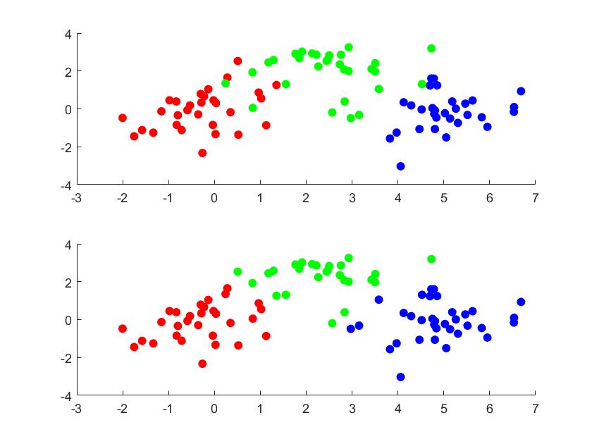
However, one can easily generalize the ratio cut to arbitrary \(k\)-partition. We define \[ \begin{equation} Rcut(A_1,\cdots, A_k)=\sum_{i=1}^k\frac{cut(A_i,\bar{A}_i)}{|A_i|} \end{equation} \] Unlike the previous methods, we define \(k\) indicator vectors \(h^1,\cdots, h^k\). For each \(h^i\), \(h^i_j=1/\sqrt{|A_i|}\) if \(v_j\in A_i\) and \(h^i_j=0\) otherwise. Let \(H=[h^1,\cdots,h^k]\) be the \(n\times k\) matrix. It satisfies \(H^TH=I_{k\times k}\). A direct computation shows that \[ \begin{equation} Rcut(A_1,\cdots,A_k)=Tr(H^TLH) \end{equation} \] Therefore, we come to the optimization \[ \begin{equation} \begin{aligned} \min\quad& Tr(H^TLH)\\ s.t\quad& H^TH=I_{k\times k} \end{aligned} \end{equation} \] By Rayleigh-Ritz theorem, the minimizer is the matrix consisting the eigenvectors corresponding to the \(k\) least eigenvalues. The last problem is that how to revert the matrix \(H\) to partitions of the graph. View \(H\) as \(n\) points in the \(k\) plane \(\mathbb{R}^k\). That is, we construct a 'dimension reduction' map \(v_i\to H_i\). Then we can cluster the points using \(k\)-means clustering.
In ratio cut, the size of partition is measured by the number of vertices. One can also measure the size by the total weights of edges. Let \(vol(A)=\sum_{i\in A}d_{ii}\). The normalized cut is \[ \begin{equation} Ncut(A_i,\cdots,A_k)=\sum_{i=1}^k\frac{cut(A_i,\bar{A}_i)}{vol(A_i)} \end{equation} \] Similarly, we define \(k\) indicator vectors \(h^1,\cdots, h^k\) such that \(h^i_j=1/\sqrt{vol(A_i)}\) for \(v_i\in A_i\) and 0 otherwise. Let \(H=[h^1,\cdots,h^k]\). Then \(H^TDH=I\), and \[ \begin{equation} Ncut(A_1,\cdots,A_k)=Tr(H^TLH) \end{equation} \] Let \(T=D^{1/2}H\) and \(L_s=D^{-1/2}LD^{-1/2}\) be the normalized graph Laplacian. We want to solve \[ \begin{equation} \begin{aligned} \min\quad& Tr(T^TL_sT)\\ s.t\quad& T^TT=I_{k\times k} \end{aligned} \end{equation} \] which is in the same form as ratio cut. To revert to the discrete case, we apply \(k\) means clustering to \(H\).
One remarkable thing about normalized cut is that it has a beautiful explanation from the perspective of random walk. Let \(p_{ij}=w_{ij}/d_i\) be the one-step transition probability from node \(i\) to node \(j\). If the graph is connected and non-bipartite, this random walk will always possess a stationary distribution \(\pi\) such that \(\pi_i=d_i/vol(V)\). Let \(P(A|B)=P(v_i\in A|v_j\in B)\) denote the probability that points in \(B\) walk to \(A\) in one step. Then \[ \begin{equation} \begin{aligned} P(A,\bar{A})&=\sum_{i\in A,j\in \bar{A}}\pi_ip_{ij}\\ &=\sum_{i\in A,j\in \bar{A}}\frac{d_i}{vol(V)}\frac{w_{ij}}{d_i}\\ &=\sum_{i\in A,j\in \bar{A}}\frac{w_{ij}}{vol(V)} \end{aligned} \end{equation} \] Therefore, \[ \begin{equation} \begin{aligned} P(A|\bar{A})&=\frac{P(A,\bar{A})}{P(\bar{A})}\\ &=\frac{\sum_{i\in A,j\in\bar{A}}w_{ij}/vol(V)}{vol(A)/vol(V)}\\ &=\sum_{i\in A,j\in\bar{A}}\frac{w_{ij}}{vol(A)}\\ &=\frac{cut(A,\bar{A})}{vol(A)} \end{aligned} \end{equation} \] We see that \(Ncut(A,\bar{A})=P(A|\bar{A})+P(\bar{A}|A)\). When we are minimizing the normalized cut we are trying to find a partition such that points have low probability that transfer from one community to the other.