Generalizations of local PCA to tangent space estimation are considered in various papers. E. Aamari and C. Levrard considered the non-asymptotic rates of local PCA in a paper of manifold reconstruction. Suppose \(n\) is the number of points and \(m\) is the manifold dimension. Then with bandwidth chosen to be \(O(\log(n)/n)^{1/m}\) the minimax rate is \(O(1/n)^{1/m}\). In their subsequent work, they considered generalization using local polynomial fitting. It happens that by involving more higher terms the convergence is faster. Suppose the fitting is up to \(k\)th term, then with the same bandwidth the minimax rate is \(O(1/n)^{k/m}\). However, they did not show practical algorithms. In an early paper of S.-W. Cheng and M.-K. Chiu, they proposed an algorithm using polynomial fitting up to the second order, but their analysis did not show consistency with the above result. However, their method is practical and its principle is easy to understand. We present a simple description in the following.
Let \(\mathcal{M}\subseteq \mathbb{R}^{m+1}\) be a hypersurface. Suppose \(x\in\mathcal{M}\) is the origin and we want to estimate \(T_x\mathcal{M}\). Firstly for the simplest case where \(T_x\mathcal{M}\) coincides with the hyperplane spanned by the standard vectors \(e_1,\cdots,e_m\) in \(\mathbb{R}^{m+1}\), we have the local parametrization \[ \mathbf{r}(u^1,\cdots,u^m)=(u^1,\cdots,u^m,f(u^1,\cdots,u^m)) \] By definition we deduce that \[ f(0)=0,\, Df(0)=0 \] Thus locally \(\mathcal{M}\) is the level set of the function \[ F(\mathbf{u})=u^{m+1}-f(u^1,\cdots,u^m)=u^{m+1}-\frac{1}{2}[u^1,\cdots,u^m]D^2f(0)[u^1,\cdots,u^m]^t+O(\|\mathbf{u}\|^3) \] We write the quadratic form in \(F(\mathbf{u})\) as the product of two vectors \[ \begin{aligned} &[\frac{1}{\sqrt{2}}(u^1)^2,u^1u^2,\cdots,u^1u^m,u^1u^{m+1},\frac{1}{\sqrt{2}}(u^2)^2,\cdots,u^2u^m,u^2u^{m+1},\cdots,\frac{1}{\sqrt{2}}(u^{m+1})^2]\cdot\\ &[\frac{1}{\sqrt{2}}\partial_1^2f(0),\partial_1\partial_2f(0),\cdots,\partial_1\partial_mf(0),0,\frac{1}{\sqrt{2}}\partial_2^2f(0),\cdots,\partial_2\partial_mf(0),0,\cdots,0] \end{aligned} \] Define \(q:\mathbb{R}^{m+1}\to\mathbb{R}^{(m+1)m/2}\) by \[ q(\mathbf{u})=[\frac{1}{\sqrt{2}}(u^1)^2,u^1u^2,\cdots,u^1u^{m+1},\frac{1}{\sqrt{2}}(u^2)^2,\cdots,u^2u^{m+1},\cdots,\frac{1}{\sqrt{2}}(u^{m+1})^2]^t \] Denote the vectorized form of \(D^2f(0)\) by \(Q_{m+1}\). Then \[ F(\mathbf{u})=\mathbf{u}^te_{m+1}-q(\mathbf{u})^tQ_{m+1}+O(\|\mathbf{u}\|^3) \] In general, let \(T_x\mathcal{M}=\text{span}\{\hat{e}_1,\cdots,\hat{e}_m\}\) and \([\hat{e}_1,\cdots,\hat{e}_m,\hat{e}_{m+1}]=P[e_1,\cdots,e_m,e_{m+1}]\). Let \(\mathbf{u}=\sum_{i=1}^{m+1}u^ie_i=\sum_{i=1}^{m+1}\hat{u}^i\hat{e}_i\). As in above \(F\) should be a function of \(\hat{u}^1,\cdots,\hat{u}^{m+1}\), here we still express \(F\) with respect to coordinate components \(u^1,\cdots,u^{m+1}\). \[ \begin{aligned} F(\mathbf{u})&=\mathbf{u}^t\hat{e}_{m+1}-q(\mathbf{u})^tq(P)Q_{m+1}+O(\|\mathbf{u}\|^3)\\ &=\mathbf{u}^tPe_{m+1}-q(\mathbf{u})^tq(P)Q_{m+1}+O(\|\mathbf{u}\|^3)\\ &=[\mathbf{u},q(\mathbf{u})]^t\left[\begin{array}{c}Pe_{m+1}\\ q(P)Q_{m+1}\end{array}\right]+O(\|\mathbf{u}\|^3) \end{aligned} \] where \(q(P)\) is an orthogonal matrix in \(\mathbb{R}^{(m+1)m/2}\).
For Euclidean submanifolds \(\mathcal{M} \subseteq\mathbb{R}^{d}\), it is similar since we have \(l=d-m\) functions \(F_{m+1},\cdots,F_d\) as above. That is, \[ F_\alpha(\mathbf{u})=[\mathbf{u},q(\mathbf{u})]^t\left[\begin{array}{c}Pe_{\alpha}\\ q(P)Q_{\alpha}\end{array}\right]+O(\|\mathbf{u}\|^3) \] for \(\alpha=m+1,\cdots,d\). Now suppose we have \(n\) samples \(X_1,\cdots,X_n\) from some distribution on the manifold. It is natural to minimize the following error \[ \frac{1}{n}\sum_{\alpha=m+1}^d\sum_{i=1}^n\left([X_i,q(X_i)]^t\left[\begin{array}{c}Pe_{\alpha}\\ q(P)Q_{\alpha}\end{array}\right]\right)^2 \] If we set \[ \begin{aligned} &A=\left[\begin{array}{ccc}X_{11}&\cdots&X_{1d}\\ \vdots&\ddots&\vdots\\ X_{n1}&\cdots& X_{nd}\end{array}\right]\\ &B=\left[\begin{array}{cccccc}\frac{1}{\sqrt{2}}X^2_{11}&X_{11}X_{12}&\cdots&X_{11}X_{1d}&\cdots&\frac{1}{\sqrt{2}}X_{1d}^2\\ \vdots&\vdots&\ddots&\vdots&\ddots&\vdots\\ \frac{1}{\sqrt{2}}X^2_{n1}&X_{n1}X_{n2}&\cdots&X_{n1}X_{nd}&\cdots&\frac{1}{\sqrt{2}}X_{nd}^2\end{array}\right]\\ &\left[\begin{array}{c}Pe_{\alpha}\\ q(P)Q_{\alpha}\end{array}\right]=\left[\begin{array}{c}g_{\alpha}\\ c_{\alpha}\end{array}\right] \end{aligned} \] it is equivalent to minimize \[ \frac{1}{n}\sum_{\alpha=m+1}^d\left[\begin{array}{c}g_{\alpha}\\ c_{\alpha}\end{array}\right]^t[A,B]^t[A,B]\left[\begin{array}{c}g_{\alpha}\\ c_{\alpha}\end{array}\right] \] Note the dimension of eigenspace of \([A B]^t[A B]\) corresponding to \(0\) can be far larger than that of normal space. Hence it works for hypersurfaces but becomes intractable for general submanifolds. Furthermore, if one writes down the asymptotic order with respect to bandwidth it is easy to notice that in fact it does not exceed local PCA. To work out a method faster than local PCA needs further consideration.
Consider the case when the number of samples is less than \(d(d+1)/2\). we add the penalty term \[ \sum_{\alpha=m+1}^d(\frac{1}{n}\left[\begin{array}{c}g_{\alpha}\\ c_{\alpha}\end{array}\right]^t[A,B]^t[A,B]\left[\begin{array}{c}g_{\alpha}\\ c_{\alpha}\end{array}\right]+\gamma\|c_\alpha\|^2) \] Then the objective function becomes \[ \sum_{\alpha=m+1}^d\left[\begin{array}{c}g_{\alpha}\\ c_{\alpha}\end{array}\right]^tZ\left[\begin{array}{c}g_{\alpha}\\ c_{\alpha}\end{array}\right] \] where \[ Z=\left[\begin{array}{cc}\frac{1}{n}A^tA&\frac{1}{n}A^tB\\\frac{1}{n}A^tB&\frac{1}{n}B^tB+\gamma I\end{array}\right]=\left[\begin{array}{cc}I&H_\gamma\\0&I\end{array}\right]\left[\begin{array}{cc}W_\gamma&0\\0&U_\gamma\end{array}\right]\left[\begin{array}{cc}I&0\\H_\gamma&I\end{array}\right] \] and \[ U_\gamma=\frac{1}{n}B^tB+\gamma I,\, H_\gamma=\frac{1}{n}A^tBU_\gamma^{-1},\, W_\gamma=\frac{1}{n}A^tA-H_\gamma U_\gamma H_\gamma^t \] Therefore, we have \[ (10)=\sum_{\alpha=m+1}^dg_\alpha^tW_\gamma g_\alpha+(c_\alpha+H_\gamma^tg_\alpha)^tU_\gamma(c_\alpha+H^t_\gamma g_\alpha) \] Note that \(U_\gamma\) is positive definite for \(\gamma>0\). Hence the minimum is achieved if \(c_\alpha+H^t_\gamma g_\alpha=0\). Let \(B=LSR\) be the SVD decomposition of \(B\). Then \[ U_\gamma=R^t(\frac{1}{n}S^2+\gamma I)R \] and \[ \frac{1}{n}B(U_\gamma^{-1})^tB^t=\frac{1}{n}LS(\frac{1}{n}S^2+\gamma I)^{-1}SL^t \] Substituting into the expression of \(W_\gamma\), we see that \[ W_\gamma=\frac{1}{n}A^t(I-\frac{1}{n}B(U_\gamma^{-1})^tB^t)A=\frac{1}{n}A^tL(I-\frac{1}{n}S(\frac{1}{n}S^2+\gamma I)^{-1}S)L^tA \] Note that the middle term is a diagonal matrix. Write \(W_\gamma=\gamma A^tL\Sigma_\gamma L^tA\). For an arbitrary element \(\lambda\in S\) it becomes \(1/(\lambda^2+n\gamma)\) in \(\Sigma_\gamma\). Therefore, the solution is given by the eigenvectors of \(W_\gamma\) corresponding to the smallest eigenvalue.
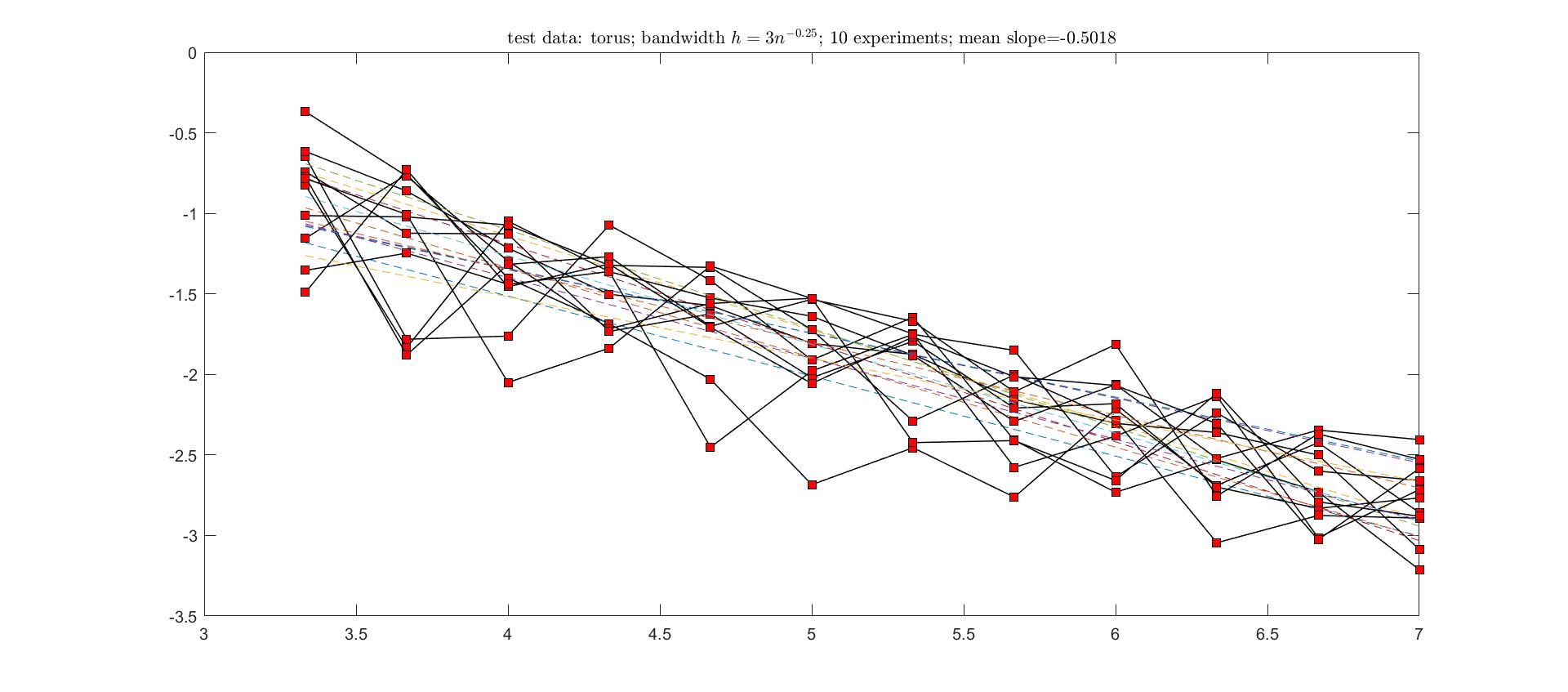
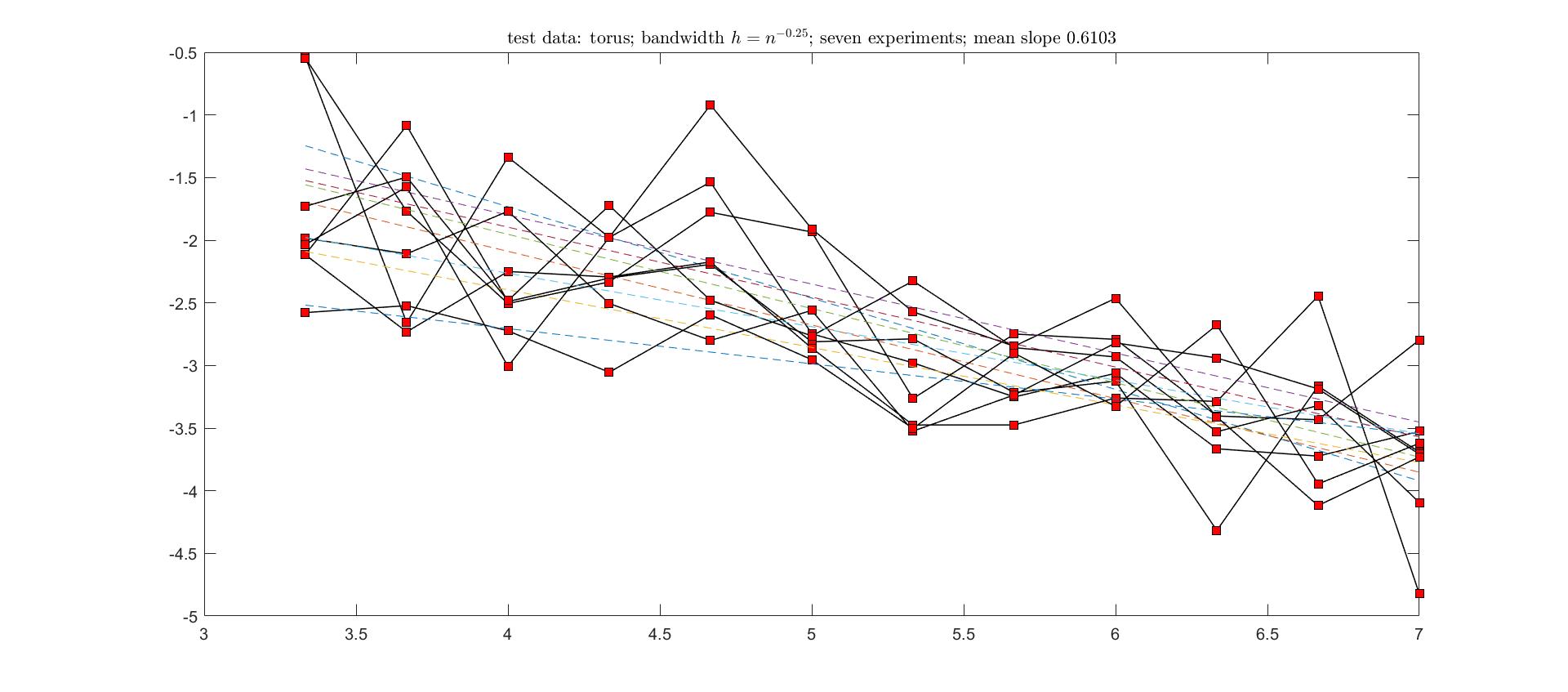
In the original paper, more techniques are involved to remove the penalty parameter and to make the computation efficient. For the convergence rate, the authors only focused on small sample size (between \((m+1)m/2\) and \((d+1)d/2\)). Under some assumptions, the angular error is \(O(h^2)\) with high probability, where \(h\) is the bandwidth. The proof involves a lot of estimations of matrix elements which are used in Gershgorin circle theorem. In fact, the paper contributes a lot to the estimation of eigenvalues. For eigenvectors they used results from relative perturbation bounds for eigenspaces, which are generalizations of Davis-Kahan theorem.