
In noiseless case we have a clean result for the convergence rate about tangent space estimation via local PCA ( see this post ). However, for noisy data the analysis is much more involved, because noise will cause points in the local neighborhood to exit, and points from the outside to enter. The integration in normal patch no more holds due to loss of true location. People proposed many practical approaches to do local PCA with the existence of noise, but few provided with a comprehensive theory. There is one method which covers both sides, called Multiscale SVD. The details are complex and can be found in this technical report, while the intuition is easy to explain and help us gain insights into other problems in manifold learning.
Let \(\mathcal{M}\subseteq\mathbb{R}^d\) be an \(m\) dimensional submanifold. Assume \(X\) is a random vector valued in \(\mathcal{M}\) with smooth density with respect to the volume measure. Let \(\eta\) be a Gaussian random vector independent of \(X\), with zero mean and isotropic covariance, i.e. \(\eta\sim\mathcal{N}(0,\sigma^2I_{d\times d})\). Consider the new random vector \(Y=X+\eta\). Then the i.i.d samples from \(Y\) are our noisy data. In noiseless case we expect to estimate the tangent space at a fixed point \(x\) from nearby samples with identical distribution as \(X\). For noisy data, however, a fixed point \(x\) on the manifold does not make sense because of noise. Instead, we are only accessible to the perturbed point \(\tilde{x}=x+\eta\), and the nearby samples are selected with respect to \(\tilde{x}\). The bandwidth, i.e. the radius of neighborhood, should be determined according to three factors:
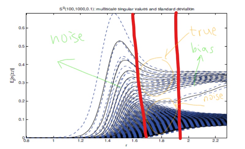
- bias: the bandwidth cannot be too large, or the nonlinearity coming from curvature will lead to terrible bias;
- variance: the bandwidth cannot be too small, or insufficient points will cause large variance due to sampling;
- noise: the bandwidth cannot be too small, or the error will be completely random due to noise.
In variance though the bandwidth is required not to be 'small', as the number of sampling increases the bandwidth does approach zero in noiseless case. This never happens when we take noise into consideration. When the bandwidth is much smaller than the magnitude of noise, the error is controlled by noise and independent to our change of bandwidth. Thus, we cannot expect a convergence by letting the bandwidth tend to zero. Accordingly, the multiscale SVD suggests us to look at the bandwidth varying in a suitable interval. This method especially works in intrinsic dimension estimation, where we need to investigate the eigenvalues of local covariance matrix. During this suitable interval, principal eigenvalues change differently from those coming from noise. Therefore, we are able to count these eigenvalues and estimate the dimension.
To understand the trade-off among bias, variance and noise, it is convenient for us to consider the following virtual case (which is also used in the analysis of multiscale SVD): suppose we first locate the nearby points and then add noise. That is, we know the true samples \(X\) before corruption. Let \(K\) be a differentiable function supported on \([0,1]\) and denote \(K_h(u)=1/h^mK(\|u\|/h)\) for \(u\in\mathbb{R}^d\). Without loss of generality, assume \(x\) is placed at the origin and \(T_x\mathcal{M}\) coincides with the coordinate space spanned by the first \(m\) standard basis \(e_1,\cdots,e_m\). Then the population covariance matrix is defined as \[ \begin{aligned} \mathbb{H}&=\mathbb{E}[YY^tK_h(X)]\\ &=\mathbb{E}[XX^tK_h(X)]+\mathbb{E}[X\eta^tK_h(X)]+\mathbb{E}[\eta X^tK_h(X)]+\mathbb{E}[\eta\eta^tK_h(X)] \end{aligned} \]
The first matrix is known to have the following decomposition \[ \mathbb{E}[XX^tK_h(X)]=\begin{bmatrix}ch^2I+O(h^4)& 0\\0&0\end{bmatrix}+\begin{bmatrix}0&O(h^4)\\ O(h^4)&O(h^4)\end{bmatrix} \] For the second and third matrix, using the independence of \(X\) and \(\eta\), they vanish in the sum. For the fourth term, using geodesic coordinates, we have \[ \begin{aligned} \mathbb{E}[\eta\eta^tK_h(X)]=c\sigma^2I \end{aligned} \] Therefore, the bias consists of two parts: the curvature of the manifold and noise. While we can eliminate the impact of curvature by choosing smaller and smaller neighborhoods, the impact of noise always exists.
Now let \(Y_1,Y_2,\cdots,Y_n\) be i.i.d. samples. By substituting the expectation by empirical mean, we obtain the empirical covariance matrix
\[ \begin{aligned} H&=\frac{1}{n}\sum_{i=1}^nY_iY_i^tK_h(X_i)\\ &=\frac{1}{n}\sum_{i=1}^nX_iX_i^tK_h(X_i)+\frac{1}{n}\sum_{i=1}^nX_i\eta_i^tK_h(X_i)+\frac{1}{n}\sum_{i=1}^n\eta_i X_i^tK_h(X_i)+\frac{1}{n}\sum_{i=1}^n\eta_i\eta_i^tK_h(X_i) \end{aligned} \] Note that \(\mathbb{E}[H]=\mathbb{H}\). For an arbitrary element in \(H\), the variance is given by \[ \mathbb{E}[(\frac{1}{n}\sum_{i=1}^nY_i^kY_i^lK_h(X_i)-\mathbb{E}[Y^kY^lK_h(X)])^2]=\frac{1}{n}\mathbb{Var}(Y^kY^lK_h(X)) \] It suffices to estimate the second moment terms, \[ \begin{aligned} \mathbb{E}[(Y^k)^2(Y^l)^2K^2_h(X)]=&\mathbb{E}[((X^k)^2+2X^k\eta^k+(\eta^k)^2)((X^l)^2+2X^l\eta^l+(\eta^l)^2)K^2_h(X)]\\ =&\mathbb{E}[\bigg((X^kX^l)^2+2(X^k)X^l\eta^l+(X^k\eta^l)^2+2X^k(X^l)^2\eta^k\\ &+4X^kX^l\eta^k\eta^l+2X^k\eta^k(\eta^l)^2+(\eta^kX^l)^2+2X^l\eta^l(\eta^k)^2\\ &+(\eta^k\eta^l)^2\bigg)K^2_h(X)]\\ =&\mathbb{E}[(X^kX^l)^2K^2_h(X)]+\mathbb{E}[(X^k\eta^l)^2K^2_h(X)]\\ &+4\mathbb{E}[X^kX^lK^2_h(X)]\mathbb{E}[\eta^k\eta^l]+\mathbb{E}[(\eta^kX^l)^2K^2_h(X)]\\ &+\mathbb{E}[(\eta^k\eta^l)^2K^2_h(X)] \end{aligned} \] The last equality holds by independence and symmetry. The order is then given by \[ \mathbb{E}[(Y^kY^l)^2K^2_h(X)]=\left\{\begin{array}{l} \frac{1}{h^m}(h^4c_1+2h^2\sigma^2c_2+4\delta_{kl}h^2\sigma^2c_2+\sigma^4c_3),\quad k,l=1,2,\cdots,m\\ \frac{1}{h^m}(h^8c_1+2h^4\sigma^2c_2+4\delta_{kl}h^4\sigma^2c_2+\sigma^4c_3),\quad k,l=m+1,\cdots,d\\ \frac{1}{h^m}(h^6c_1+h^2\sigma^2c_2+h^4\sigma^2c_2+\sigma^4c_3),\quad \text{otherwise}\end{array}\right. \] Thus with high probability, \[ H=\begin{bmatrix}ch^2I+O(h^4)+O(\frac{h^2+\sigma^2}{\sqrt{nh^m}})& 0\\0&0\end{bmatrix}+\begin{bmatrix}0&O(h^4)\\ O(h^4)&O(h^4+\sigma^2)\end{bmatrix}+\frac{1}{\sqrt{nh^m}}\begin{bmatrix}0&O((h^2+\sigma^2)^{3/2})\\O((h^2+\sigma^2)^{3/2})&O(h^4+\sigma^2) \end{bmatrix} \] If \(\sigma \ll h^2\), then the error is mainly controlled by bandwidth and the noise is relatively negligible. If \(\sigma\gg h^2\), the error largely depends on noise. Define \(\gamma=\sigma/h^2\). Then \[ \frac{1}{h^2}H=\begin{bmatrix}cI+O(h^2)+O(\frac{1+\sigma\gamma}{\sqrt{nh^m}})& 0\\0&0\end{bmatrix}+\begin{bmatrix}0&O(h^2)\\ O(h^2)&O(\sigma\gamma)\end{bmatrix}+\frac{1}{\sqrt{nh^m}}\begin{bmatrix}0&O(\sigma^2\gamma)\\O(\sigma^2\gamma)&O(\sigma\gamma) \end{bmatrix} \] If \(\sigma\ll \sqrt{nh^m}\), then the error is at least \(O(\sigma\gamma)\) and one cannot get better result using local PCA. If \(\sigma\gg \sqrt{nh^m}\), then the situation is terrible with large noise and inadequate sampling, with error in the order \(O(\sigma^2\gamma/\sqrt{nh^m})\).